Trevor Nagel

Earlier this month I decided to rework the back end of the renderer to improve performance on lower spec machines.

I made the following changes:

• Visibility buffer has been removed. I had conceived of the visibility buffer sometime ago when counting the prohibitive cost of overdraw in the shaders. It was a decent solution, but represented too much overhead for what it saved.
• Hierarchical z buffer replaces the visibility buffer. This is the depth buffer expressed as a tiled hierarchy of maximum depth values to allow for the early z reject of whole tiles in the rasteriser.
• Single pixel shader. Previously a triangles’ pixel shader was a series of function pointers to small shader code blocks. I had thought about using ASMJit or LLVM to output some machine code and stitch it together, but felt I needed a more simpler sort term solution. So now every game surface has the same shader applied: a perspective correct 3 channel colour pass and a point sampled mip-mapped texture pass. The renderer now expects the same attributes and shading pathway for every scene triangle. This simplified code flow in the back end

The hierarchical z buffer has the following constituents:

• Level 0 is the native tile depth buffer containing the current scene depth per pixel
• Level 1 records maximum depth for each 4×4 tile
• Level 2 records maximum depth for each 16×16 tile
• Level 3 records maximum depth for each 64×64 tile
• 2 x 64-bit masks for tracking writes at level 2 & 3

Depth writes from valid triangle fragments must be propagated up the hierarchy, which is handled as follows: for each fragment that writes to level 0 the shader returns a maximum depth value for the 4×4 pixel block, which is written into level 1. The level 2 & 3 tiles this block resides in are bit-marked.

After all the fragments from a triangle have been shaded the level 2 then level 3 depth tiles whose bits are set in their respective masks are updated by writing up maximum values for each 4×4 block. SIMD is used to accelerate the process.

In the rasteriser we step interpolated depth values from tile corners using pre-computed step tables in the same way we step edge values. By taking the minimum depth for the 4 corners of each tile we have a conservative depth value for the raster tile which can be compared to the corresponding depth tile entry. If the minimum raster depth in that tile is less than the maximum buffer depth we can trivially reject the whole tile before it is emitted to the fragment stream.

The depth buffer hierarchy is cleared following bin processing.

Depth interpolant setup is done in the tiles ahead of rasterisation using SIMD to process 4 triangles at a time. A real win has come from the deferred nature of the binned renderer: if no triangle fragments survive rasterisation then we avoid attribute fetch, attribute shading and vertex lighting calculations for that triangle completely!

The hierarchical depth buffer’s effectiveness hangs largely on the order triangles arrive at the buffer. You want to process them front to back ( closest to the camera first) to get the most out of it. I considered briefly doing a full per-triangle depth sort in the bins but quickly discounted it. Even with the modest scenes Lamorna Engine is intended to handle that could mean sorting thousands of triangles at a time. And I reasoned it was unnecessary to sort triangles, only models. Since triangles in the bin are laid down according to draw call, I implemented a draw call sort, then ensured that lower numbered draw calls contained large occluding models such as the map elements. I also depth sort the animated models prior to rendering as well, since they have the highest poly counts.  

I am really impressed with the effectiveness of the hierarchical depth buffer. Not only did it not take long to implement, but it gave a large performance boost on lower spec machines.

I have a number of dev machines for testing purposes, and my low spec one is a dual core Core i5 2.3Ghz 4Gb HP laptop, circa 2011. Previously versions of the demo have run very choppily on this machine, 30-40 fps, but with the new changes the demo barely drops a frame below 60.

Happy days!

This is part of a series about the different game systems I’ve created for Lamorna Engine.

Lamorna engine features a basic sound engine that handles basic 2 channel spatial audio, with multiple sound sources mixed into a local buffer and streamed to DirectSound.

The sound system is composed of a number of elements:

• Sound file: these contain the raw sample data. I target the sound files used by the original Quake game, which are 8-bit, 11 Khz .wav files. This is a low quality, low bit-rate format but proves adequate for my needs. Internally these are converted to 32-bit prior to mixing. The .wavs are loaded at setup.
• Sound trigger: contains a list of sound events initiated in current frame. The sound trigger sub-system parses the ECS for entities with a ‘sound’ component and checks for sound events, usually triggered by state changes. It also checks the collision system output for collision events that emit sounds not associated with entities such as projectile impact. Each sound source has a unique source id indicating its origin.
• Active sounds: an active sound entry contains an index into its source .wav file, a current play cursor, source id, and left & right volume values. The active sound manager maintains a list of active sounds. Newly triggered sounds are added to the playlist and sounds that have finished playing are removed.  The id of incoming sound triggers are checked and should a new sound match one currently playing the sound is simply restarted.
• Local mixing buffer: the active sound list is processed each frame and sufficient samples generated to fill a local buffer. This buffer is written down to the DirectSound buffer initialised at setup. This buffer is in 2 channel 32-bit float format.
• DirectSound buffer: The final destination for our sound samples is the Directsound buffer. This is initialised at setup and set playing, after which it must be kept supplied for smooth sound delivery. It’s operations are handled by the OS and is opaque save for a play and write cursor whose positions can be queried. The buffer must be unlocked and then locked following write operations.

The process of generating sound samples each frame focuses on the active sound list.

The source position of each active sound is transformed into camera space and left and right volume values computed based on orientation, and attenuated by distance into a linear soundscape with a near and far plane for clean cut-off.

Sound samples are generated for each sound and mixed into a local buffer. The raw .wav format is 8 bit mono, so the samples are converted to 2 channel 32-bit float and attenuated by the volume calculated earlier. The generated samples are summed into the buffer and clamped to prevent overflow. This is all done using SIMD, processing 4 samples at a time.

Possibly the most difficult aspect of creating a sound system is properly filling the DirectSound buffer, determining how many samples to write at a time and how often. I understand a common method is to fill the buffer a certain amount then initiate a callback for when the buffer needs refilling, but I took a different approach. I write to the DirectSound buffer each frame, and oversupply by a conservative amount. In the following frame I check how many samples have actually been consumed and advance my active sound play cursors by that amount. I considered this a simpler approach, and by oversupplying slightly you cover any irregularities caused by system lag, albeit at a slightly higher processing cost.

A couple of other points to note:

• Sounds can marked as looping, in which case the play cursor is just reset at the end of the file.
• Ambient sounds are excluded from spatial computations
• In the cases where a sound does not match the duration of a sound event  I use a small null sound to cut the sound off. The doors are a good example of this

Thank you!

This is part of a series about the different game systems I’ve created for Lamorna Engine.

Lamorna engine features dynamic lightmaps, which allow for the real time world painting effect. The light maps are low resolution textures of uniform texel density applied to static world surfaces, which can accumulate colour from light emitters. Each surface of the blocks that make up the game world are assigned a unique texture at setup, and the deltas necessary to map from world coordinate space to local lightmap space are stored. A base texture is applied to the lightmap, since this is the only texture applied to the surface some visual detail is necessary, and colour is accumulated over this base texture. Mip-maps for the lightmaps are also generated.

The process of updating the lightmaps each frame begins by determining which light emitters are casting light on which world blocks. This process is accelerated using the bounding volume hierarchy created for collision detection, where the static world blocks have been binned to a bounding grid at setup, partitioning up the world into nodes which can be checked and trivially rejected. Since both the nodes and the world blocks are axis aligned, a simple overlap test against the light volume suffices. We use SIMD to process firstly 4 grid nodes at a time, then 4 bounding boxes, and sparse array compression to output an indexed list of lit surfaces vs light sources.

The narrow phase processes each lit block with a list of valid light sources close enough to contribute colour, where each light source has a position, colour and intensity. The modus operandi of the algorithm is to compute a colour contribution from the light source for each lexel (lightmap pixel) in the lightmap based on the distance to the light source and its intensity. Instead of a radiosity calculation per lexel the process contributes colour to a surface by way of a projected texture light. This is a grayscale texture that describes light intensity fall-off in 2D :

If we imagine instances of this texture lying on the plane of each of the principal axes and centred at the light source, we can see a 3D position in world space can be mapped into this texture to obtain a light intensity value, where the z component is used to attenuate the u, v components. This is similar to the process Doom 3 used for it’s real time lighting, and is a neat way of avoiding complex radiosity calculations while giving artistic control over light properties, particularly fall-off. To avoid having to visit each lexel on the surface we compute a bounding rectangle for the light’s extent in lightmap space, clamp it to the lightmap dimensions and iterate within it. Lights that lie behind the lightmap plane are skipped. Lighting computations are performed on the highest mip level. Once all the lights affecting a surface have been processed the lower level mip-maps are re-computed.

The narrow phase is threaded, where each lit block and it’s attendant light sources are expressed as a job and submitted to the thread pool. The whole lightmap scheme is double buffered with read & write copies of each lightmap, so that the renderer can access the read copy while the write copy is being updated. To maintain continuity the write process must copy over the read lightmap before updating begins. At the end of the frame the read and write references for those lightmaps that have been updated are exchanged. The double buffering doubles the memory requirements but allows us to run lightmap update in parellel with rendering, albeit at the negligible cost of lagging one frame behind the world update.

The dynamic lightmaps are used to create a permanent ‘painted’ effect in the game world, but could just as easily be used for dynamic lighting by resetting the lightmaps each frame. The lexel to world space ratio can be adjusted, with higher ratios improving visual fidelity at the cost of performance.

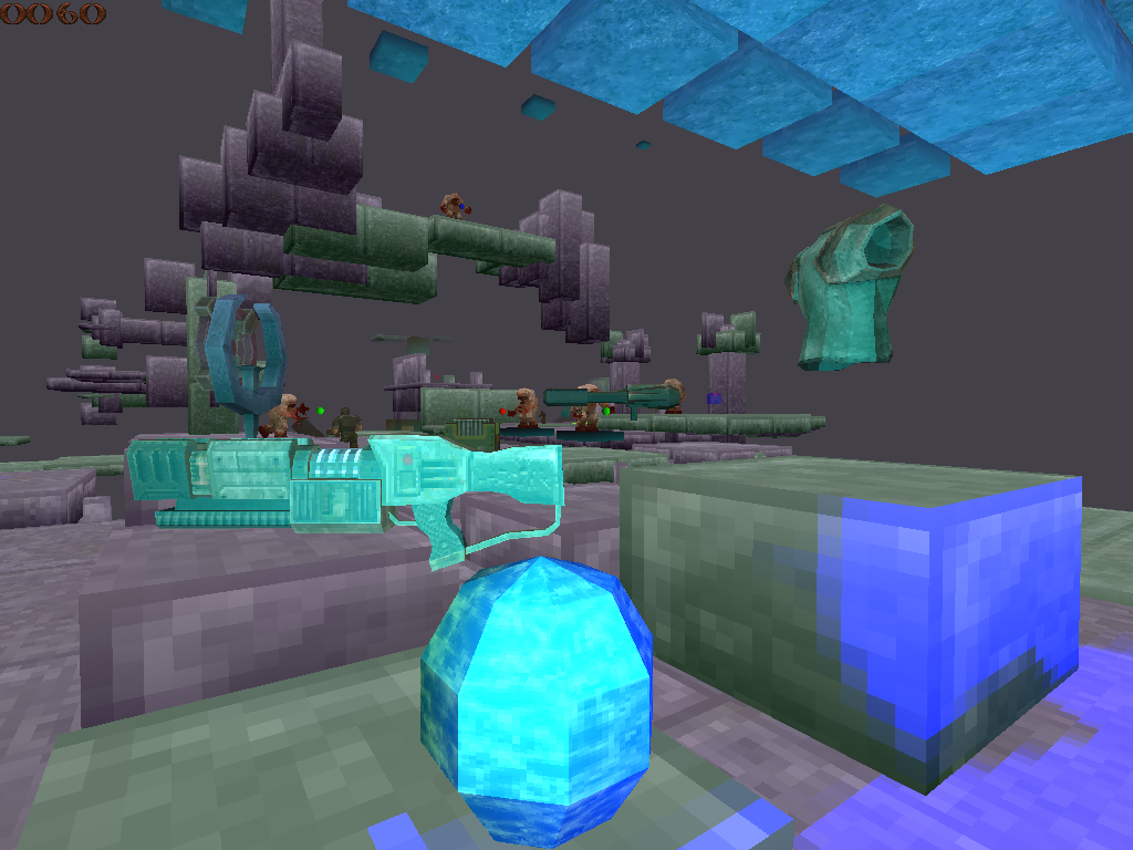
Lamorna engine has a simple but robust collision scheme. Simple, in that it only supports linear collisions against axis aligned surfaces, but robust in that it uses an internal fixed point format to give strong guarantees about precision. The process is multi-threaded, and uses a broad phase check against a bounding volume hierarchy (BVH) to quickly discard non-colliders.

I found collision detection one of the hardest game systems to write, even more so than rendering. Whereas the occasional graphical glitch may be tolerable, collision is unforgiving; pushing through a wall or falling through the floor is a deal breaker for player experience. It wasn’t until switching to a fixed point solution that I was able to completely eliminate the occasional collision failure.

Colliding entities are expressed as axis aligned bounding boxes, with a position and extent. This makes a preliminary overlap test as simple as checking the sum of the extents against the absolute difference between the two positions for each axis. The position and extent are in 16:16 fixed point format, with all calculations being done in 64-bit. The collision system defines colliders and collidees, where colliders are dynamic elements like players, monsters, projectiles and such, and collidees are the mostly static world elements. They are identified in the ECS with respective components. Some of the moving elements are both colliders and collidees, the players and monsters for example. For some elements like the blocks that compose the game world, the bounding box is a direct expression of it’s shape, for other more complex models it is simply an approximation. The collision system’s modus operandi is to take each collider in turn and collide it against each collidee that falls within it’s purview, adjusting the position of the collider as needed, but treating the collidees it encounters as static. This makes for a straightforward scheme, and works perfectly for simple collision encounters such as player vs static world, projectile vs moving entity, but starts to break down when more complicated interactions between two or more moving objects are required.

Pre-process

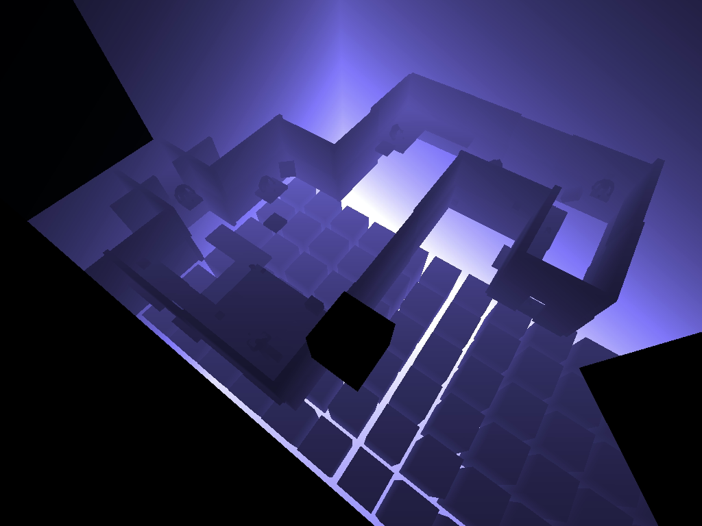
The collison process opens with a pre-step that bins all dynamic collidees into the static collidee BVH. This static BVH was created at setup by binning all static world elements into a regular 3D grid, and then adjusting the bounds of each node of the grid to fully contain it’s set. This loose grid approach creates nodes of differing sizes but means each colliding element is present only once, which I felt was a win over a tight BVH where collidees spanning multiple grid nodes are duplicated across those nodes. There are not nearly as many dynamic collidees needing binning in comparison to static collidees, so the run time binning is not particularly time consuming. The grid nodes are re-adjusted each frame to fit the included dynamic collidees. The entries in the BVH include references back to the source entities in the entity-component system (ECS).  

Broad Phase

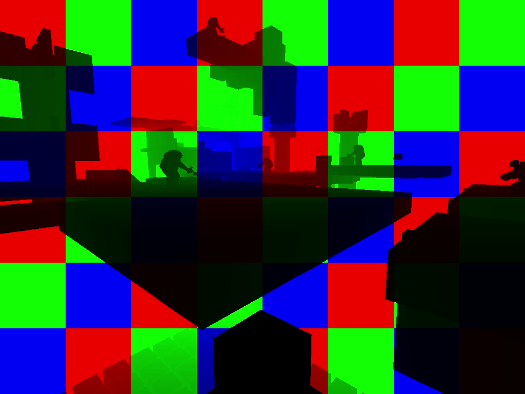
The next step is the broad phase, which checks each collider against the BVH, using a conservative bounding box that contains the extent of the collider’s potential movement during collision, and outputs a list of potential collidees for narrow phase analysis. We use SSE to process firstly 4 grid nodes at a time, then 4 bounding boxes, and sparse array compression to output the final index lists.

Narrow Phase

The input into the narrow collison phase is a list of colliders each with an array of potential collidees, those colliders with no potential collidees having been excluded. Each collider has a position, a movement vector and colliding extent, now expressed in fixed point format, and each collidee a position and extent similarly expressed. The narrow phase is iterative, checking the collider against each potential collidee in turn, adjusting it’s position and direction, then re-checking until it’s movement vector is consumed, no more collisions are detected or an upper iterative bound is reached.

Collision checks in the narrow phase are performed by expressing the collider as a point and directed line segment and the collidee as series of axis aligned slabs, with it’s extent expanded by the extent of the collider. Intersection intervals are generated for the line segment against each axis slab, and composited into a final interval for each bounding box, the smallest valid one being the collision interval for the set. The collider’s position is then stepped to the intersection point using this interval.  For more details please see Christer Ericson’s excellent text ‘Realtime Collision Detection’, in particular section 5.3.3 ‘Intersecting Ray or Segment Against Box’. 

Working with axis aligned boxes means the collider’s position can be clamped to the colliding axis, offset by a small epsilon to push it off the surface, which is a big aid to fidelity. The movement vector of the collider is adjusted, depending on the type of collision response required. For deflection, which yields the sliding behaviour you want for natural moving entities like the player and monsters, the movement vector is set at a tangent to the colliding surface. For reflection or ‘bouncing’, the movement vector is reflected about the surface normal. The collider can also be brought to a stop by the collider, in which case the movement vector is set to zero. The type of collision response for the current collider-collidee pair is obtained from a look up table. The movement vector is expressed as a normal vector and magnitude. I found this approach easier to work with, and more robust. ‘Consuming’ the movement vector as the collision steps proceed becomes simply a case of decrementing the magnitude, and the normal vector can be clamped to an axis without a loss of precision.

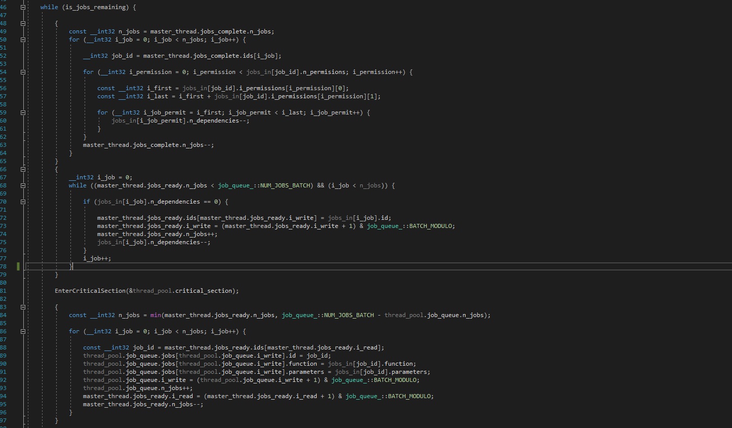
The narrow phase collision process is expressed as a series of jobs fed into the thread pool, where a worker thread is handed a collider and it’s list of potential colliders. The output is a list of valid colliders and collidees with their contact points, which can be parsed by the game logic systems for further collision outcomes.

The only non-axis aligned elements in the game world are the bounce pads, which are treated as an axis aligned box in a coordinate space described by 3 basis vectors that orient the box. Collision proceeds as per usual save colliders are mapped into this coordinate space prior to collision checks. This process hasn’t been as stable as the base one in the past, and I haven’t been confident using oriented surfaces for generalised collisions.

As a final point, some game entities need to be able to step or rise over low obstacles for continuity of motion. This is done by running a second narrow phase collision pass for a slightly elevated copy of the collider, and if that copy can proceed where the original is blocked the entity is allowed to surmount the collidee.

Please check out my previous posts on other game systems.

Let’s start with some definitions:

Entity: anything that exists in the game world, either visible or invisible e.g. player, tree, trigger box, patrol way-point. A sound is not an entity, but a sound source could be

Component: a discreet property of an entity that contributes to describing its presence in the game world e.g. position, velocity, colour. Components can be of varying granularity, a ‘camera’ component could contain various sub-components such as matrices and vectors describing the camera orientation, or a component could be a single element like ‘speed’

An entity can be thought of as the sum of its components

Systems: processes that operate on an entity’s components e.g. rendering system, collision system, sound system. They typically read in component data, perform a transform on it and write the result back

ECS: entity-component system. A conceptual model that defines relationships between entities, components and systems. Computer games are at their core about interactions between entities. These interactions can be irregular and complex. “This lever opens a door 50 metres away which lets out a cat that in 30 seconds will turn into a flying carpet the player can ride”. Developing a system that can properly handle such complexity is an open problem. An ECS is one of many approaches, it makes components first class citizens stored in a flat database like structure, and entities just an implicit and mutable collection of components. Game systems know nothing about what entities they are operating on, only their components.

Lamorna Engine’s ECS is loosely based on the one employed by the Unity game engine: https://www.youtube.com/watch?v=p65Yt20pw0g

In a classic ECS game entities are fully dissociated into components distributed across a large database. My approach takes a step back from this and attempts group entities with the same components together in order to be able to do indexed iteration on components. In line with the Unity approach these groups are called archetypes, and represent what would conventionally be an object type like a monster or weapon.

Components are simply structs with a small number of member components. The granularity of the components really depends on needs and circumstance, but as a general rule a components should have a small and directed number of members. Each component has an ID and it’s size is known for memory allocation.

Archetypes have a bit-mask identifying what components they contain, an entity count, and the component arrays. Within the archetype entities exist implicitly as an index into the component array. Each has a component bit-mask, allowing us to toggle components on and off at run-time using a simple bit operation. Entities can not be assigned additional components at run-time beyond what they are initialised with, but their existing components can be disabled and enabled. So for example the ‘collide’ component can be disabled to exclude an entity from collision checks temporarily.

Engine system functions are given a list of components to operate on. In a preliminary step the function parses the archetype list for archetypes containing the components it seeks, and returns pointers to the start of each component array for each valid archetype. These can then be iterated over with an index in the familiar manner. The component bit-mask used to match archetypes is also checked against each entity’s component mask. Thus archetypes containing system components are discovered, but individual entities with one or more of those components toggled off will be ignored.

There is some overhead in operating an ECS. In my version system functions are run cold each time, that is with no assumed knowledge of which archetypes contain which components, so the pre-process described above is run each time the function is called. However what we lose with this added complexity we gain by making functions wholly entity agnostic. Adding a new component to an archetype adds all it’s functionality without having to touch any system code. Decide that you want an entity to fly? Drop in the ‘fly’ component and providing you’ve done your work right the entity will fly.

AN ECS takes time to implement and balance but when set up it can be very powerful. It forces you to be rigorous in defining the boundaries of system functionality, and component scope. My approach has undergone a few iterations but is still in some flux, I’m find myself having to create components as simple identifiers as an aid to game systems, which seems to indicate that further refinement is needed.

ECS is in truth an overkill in a game engine as simple as Lamorna, however it was a good learning experience writing it.

Read about the front end of the renderer here.

The front end or geometry stage of the renderer finishes with all valid scene triangles having their screen space coordinates written to the buffers of the screen bins they cover, where a valid triangle is one that is front facing, has pixel coverage and lies within the view volume,

The back end of the renderer has a series of distinct stages:

• Visibility buffer fill
• Visible triangle atrribute fetch and shading
• Visible fragment pixel shading

Visibility Buffer Fill

Triangles are fetched from the bin buffer and rasterised into a stream of raster fragments. For more details on this see the post on the rasteriser.

Those fragments that survive the depth test write into a visibility buffer, analogous to the other screen buffers such as depth and colour, except into this buffer we write a 32-bit value that uniquely identifies the triangle, and maps back into the triangle’s bin entry, which in turn indexes the parent triangle’s vertex data. Once all the bin triangles have been processed this buffer contains the id’s of all and only the visible triangles in the frame.

Visible Triangle Attribute Fetch & Shading

The visibility buffer is parsed a row at a time, leveraging spatial coherence by writing out edge pixels, removing duplicates, and checking against existing ID’s stored in a hash table.  The output of this process is a list of visible triangles grouped according to draw call.

The list is stepped through and for each triangle attributes are fetched and shaded. Attribute shading consists of multiplying by an attribute matrix, or applying some basic vertex lighting. Attribute deltas are computed for barycentric interpolation in the shader. The rasteriser is re-run for each triangle, but this time instead of using the depth buffer as a write mask, the visibility buffer is used. The raster fragments are fed into the pixel shader.

Pixel shading

Lamorna engine’s pixel shading is fairly simple in it’s scope. It can perform perspective correct 3-channel colour interpolation and perspective correct point sampled texture mapping with per fragment mip-mapping, where in my parlance a fragment is a 4×4 pixel block, with either clamp or wrap.

The shading process proceeds a fragment at a time, and opens by stepping the edge values emitted from the rasteriser to the pixel centres, and multiplying through by the inverse of the triangle area to yield the normalised screen space barycentrics. These barycentrics are used to step 1/z depth across the fragment. A second set of barycentric coordinates now come into play. These barycentric coordinates were assigned in the front end and underwent clipping, projection and binning along with the position coordinates. Interpolating these across the fragment and dividing by the depth yields barycentric coordinates for the current pixel in the original clip-space triangle, which allows us to interpolate un-clipped and un-projected vertex attributes from that point on in the shader.

Once all the visible triangles have been shaded the bin colour buffer contains the final output of that bin for the frame.

While the whole screen is divided conceptually into 128×128 pixel bins, there are in reality only as many bin buffers as there are worker threads. When a thread has finished processing the contents of a bin, the bin colour buffer is written down to the DirectX surface buffer.

Each 64×64 tile within the screen bin is mapped using morton coding to improve memory access patterns, so the colour buffer is swizzled during copy down. All buffers are cleared ready for the next bin.

Considerations:

• The visibility buffer complicates the rendering process but is intended to remove the effects of overdraw in the pixel shaders. It allows attribute fetch, shading and pixel shading to be wholly limited to visible triangles.
• The hi-jinks with the two barycentric types is in part necessitated by the deferred pipeline. Attributes need to be either clipped explicitly after fetching which would be messy, or implicitly via the clipped barycentrics.
• The shaders make heavy use of SIMD, processing 4 elements at a time. The lack of a feature complete vector ISA hurts here, as things like texture reads and computing mip-map levels must be done using scalar code.
• I find it necessary to clamp u & v values in the shader to prevent the occasional bogus texture read.
• Draw calls are used to group models having similar pixel shading routines.
• I have in the past implemented tri and bi-linear filtering, and texture blending, but they led to unacceptable performance degredation.

Lamorna Engine features a software rendering pipeline. It has a sort middle architecture, where triangles coming off the geometry stage are binned prior to further processing. The following is brief description of the process.

Triangles are submitted to the front end of the renderer as part of a draw call containing index and vertex lists for models that share a common back end shading routine.

• The renderer processes triangles in batches, 16 at time, and starts by filling a vertex buffer with unique triangle vertices, maintaining an internal index list to avoid duplicating vertices shared amongst the batch. This process takes the place of a vertex cache.
• Vertices are shaded, which is a rather euphemistic way of saying to say they are transformed by a composite of the camera, model space and projection matrix into clip space. Only position vertices are fetched by the front end, attribute fetch being deferred to the back end.
• The clip space vertices are checked against the view volume and clip codes generated, bit masks marking vertices as either inside or outside the volume.
• The vertices are explicitly assembled into triangles using the index list, and barycentric coordinates assigned. Triangles whose vertices lie wholly outside the view volume can be discarded.
• Triangles that intersect both the view volume and the guard band have their vertices, including barycentrics, clipped against the relevant planes. Triangles coming off assembly and clipping are accumulated.

Once enough triangles are accumulated the second stage of the pipeline is run.

• Triangle vertices are projected by dividing through by their depth, and mapped into screen space.
• Triangle area is computed and a bounding box generated for binning. The triangle vertices are snapped to 24:8 fixed point format ahead of area and bounding box computation, and the area computed in 64-bit to avoid overflow. The sign of the area is used to exclude back facing triangles, and the bounding box to exclude co-linear triangles, and those with zero pixel coverage.
• Triangles that survive this culling process are written into the screen bins they cover by walking their bounding box over the bin array. Triangles have their screen space and barycentric coordinates copied to each bin their bounding box covers, along with indices to their parent vertex & model list.

Processing a draw call is expressed as a job for the thread pool. Each thread owns a copy of the screen bin structure so it can run without a need for synchronisation. At the end of draw call processing all valid triangles have been binned across a 3 dimensional array of form [i_thread][tile_x][tile_y]

Considerations

• The process makes use of SSE to process 4 elements at a time, transposing components into ‘structure of array’ format ahead of computation blocks.
• The triangle batch is expressed as a circular buffer with a virtualised index as described by Fabien here .
• The guard band is an expression of the precision limits of the fixed point format used in the rasteriser. I approximate this limit in clip space by scaling out the view volume.
• Lamorna engine defers attribute fetch till just prior to pixel shading. This necessitates sending clipped barycentric coordinates through from the front end for use as attributes in the shaders.

Till next time!

Rasterisation is the process of determining screen pixel coverage for a triangle. Lamorna engine’s rasteriser uses the concept of half spaces, where each triangle edge divides screen space into an inside and outside half, and evaluating the edge equation at a pixel centre can determine which half it lies in. The pixels we are interested in lie within the intersection of the 3 inside half spaces of the triangle. A brute force approach to testing pixels would be to traverse the triangles bounding box, but more sophisticated techniques that try to do less work exist, one of which is the hierarchical descent method, which divides the screen up into a tile hierarchy, and tests tiles before pixels, hoping to quickly exclude blocks of pixels that lie outside the triangle, and include blocks of pixels that lie within. This was the approach taken by the Larrabee engineers and Lamorna engine tries to tread the same path.  That article does a much better job of describing the nitty-gritty of the process than I could, but suffice to say that for each triangle we use the edge equations to generate step tables for each edge and recursion level sufficient to allow us to step into a 64×64 tile processing pixel blocks at a 16×16 and 4×4 level, rejecting and accepting blocks as we descend. Each block has a reject and accept corner, corners which are closest and farthest from the edge respectively. A typical triangle will have larger blocks accepted in it’s interior, while around the edges the routine will descend into 4×4 tiles emitting pixel coverage masks.

Lamorna engine partitions screen space a couple of ways. The first partition is a bin, a 128×128 pixel boundary. This division serves the front end of the renderer, where triangles coming off the geometry staged are explicitly assigned to the bins they overlap by copying to an associated bin buffer. The bins are about cache friendliness and division of thread labour. Within the bin, screen space is further divided into four 64×64 tiles, which are the targets for the rasteriser.

The rasteriser fetches a triangle’s binned screen space vertices and snaps them to 24:8 fixed point format. We allow 8 bits of sub-pixel precision as per the DirectX spec. Edge deltas are computed along with the triangle area in 64-bit space to avoid integer overflow. A bounding box for the triangle is computed. Triangles whose bounding box covers 4 pixels or less are sent to a dedicated small triangle rasteriser which skips step table setup and calculates edge values directly at pixel centres.

For remaining triangles the rasteriser visits each 64×64 tile in the bin evaluating the edge equation at tile reject and accept corners in 64-bit. If a whole tile can not be trivially accepted or rejected the starting edge values seed the descent into the tile hierarchy. We add the edge value to our reject step table values and generate a bitmask result for each of the 16 sub tiles, with a bit set for each tile that is rejected. We then add the accept step table and generate a second bit mask. We use SIMD to process blocks 4 elements at a time. The edge equations are set up such that negative edge values denote the inside of the triangle, so bitmasks can be built directly off of the sign bit. Bit operations sum the results for each edge into a composite mask which can be scanned to obtain the trivially accepted and partially accepted blocks. The lowest level of recursion steps edge values from the corner of a 4×4 block to the 16 pixel centres and emit a pixel coverage mask.

Proper tie-breaking rules for pixel ownership must be considered, so adopting DirectX standards we displace the bottom-right hand edges ever so slightly as described by Fabien . This edge bias is applied once per edge during step table setup to the lowest level of the reject table which steps to pixel centres.

The process described in the Larrabee paper disconnects rasterisation from shading but Lamorna engine tasks the rasteriser with emitting barycentric coordinates to the shaders so must needs descend into trivially accepted blocks as well as partially accepted ones.

The final output from the rasteriser is a small data structure that for each 4×4 block touched by the triangle contains 2 starting edge values, an offset into the tile buffer, and an optional coverage mask. The rasteriser processes a triangle at a time, outputting a stream of draw commands to the shader. So rasterisation and shading proceed one after the other, a triangle at a time.

A pre-shader process uses the step tables from the rasteriser to step the 2 edge values to pixel centres for each 4×4 blocks and multiplies thru by 1/triangle area to yield the normalised  barcyentric coordinates. Triangle attributes such as depth and texture coordinates can then be computed. 

Considerations

• Rasterisation is a real pain to get right! There are a number of gotchas sorrounding the fixed point format and precision limits.
• Rasterisation origin is set to the bin centre to maximise bit precision.
• Triangles that exceed the limits of the fixed point format must be clipped. 
• Care needs to be taken when working with the fixed point format. It’s important to be aware of overflow and rounding error. I found the MSDN data conversion rules here helpful in getting consistency in moving between representations.
• Edge tables are in 32-bit fixed point format, keeping them that way is essential to be able to leverage the power of SIMD.  However there are limitations on the size of tile that a triangle can be rasterised to using 32 bit step tables. This limit seems to be 64×64 pixels.
• I found very small triangles caused problems for the hierarchical rasteriser. The geometry stage rejects small triangles that don’t have any pixel coverage, but those that do can be so small as to not generate sufficient bits to step accurately from tile corners. Hence the small triangle rasteriser.
• Starting edge values for each tile end up being in 16:16 format, as they are the products of 24:8 numbers. Fabien points out that these extra bits can be discarded without loss of precision (see comments), so the result can fit in a 32-bit integer. 
• Nicholas Guillemot has a collection of notes on rasterisation that are helpful.

Till next time!

 

Lamorna Engine features a hand made thread pool with a work queue that supports the notion of job dependencies.

A job consists of the following elements:

• pointer to the function to be executed
• pointer to a struct containing parameters to that function.
• dependency counter, indicating how many jobs it must wait on before running
• permission list, indicating which jobs are dependant on that job’s completion.

All jobs with dependencies > 0 are placed in a ‘pending’ queue. As jobs finish they decrement the dependency counter of the jobs in their permission list. When a job’s dependency counter reaches zero, it can be added to the ‘ready’’ queue.

The worker threads are created at start up and promptly slept until signalled by the master thread that jobs have been added to the ‘ready’ queue. A worker thread wakes in it’s critical section, takes a job from the ‘ready’ queue, exits the critical section and executes the job. When done it re-enters the critical section, adds the job to the ‘finished’ queue and selects another job, or sleeps if there are none.

It is the job of the master thread to keep the ‘ready’’ queue full. It wakes when that queue is not full, processes the ‘finished’ queue, adding any jobs that now have zero dependencies to the ‘ready’ queue. When all jobs are complete control returns to the master thread.

Naturally a batch of jobs submitted to the thread pool must have at least one job with zero dependencies which will kick off the process.

The above is based on an approach I read about here by Charles Bloom

Using the above I can characterise an entire game frame as a single large submission to the thread pool, expressed as a network of interdependent jobs. This certainly isn’t to say those dependencies are highly optimised, in fact large sections of game logic still run serially due to the difficult nature of parallelising such work, but it is all still expressed using the same scheme. Rendering, dynamic lightmap generation and collision processes are all highly parallelised.

Lamorna engine makes use of what I style a command buffer to aid with parallelisation. At the end of each frame the details necessary to render each visible model; position, scale, rotation matrices etc are written to a command buffer. This data is double buffered, so the renderer can be working on the previous frame’s command data while the current frame is being populated. In addition to rendering data, sound and lighting data are also written down so audio and lightmap generation can be run concurrently as well.  

The queues are implemented as ring buffers with virtualised indices as described in Fabien’s excellent article. 

The number of worker threads is set to match the number of processors on the machine.

Improvements: I recently became aware of lock-free synchronisation after reading about it in the text ‘Concurrent programming on Windows‘, and following that up by watching Casey Muratori’s thread work on Handmade Hero. I’d like to explore that as an alternative to critical section entry, but truth is I’m not sure how much difference it would make. From what I understand a thread attempting to enter a critical section will spin-wait for a bit anyway before being switched out. The time spent in the critical section for each worker thread should be minimal, since it just writes down it’s completed job and picks up another.

Till next time!